
Why does Nf3 Score Better?
In the Lichess database, 1. Nf3 scores better than 1. e4. Is that a matter of chess, or statistics?

In my previous post, I looked at how we could estimate how choosing an opening move with a higher database winrate would affect a player’s rating. As a running example, I compared e4 and Nf3.
On reddit, most comments concerned the foundational observation, that Nf3 has a higher winrate than e4.
One comment in particular claimed that the whole thing was just a statistical quirk, and Nf3 doesn’t really outperform e4 at all:
This is Simpson’s Paradox. Dive into Nf3 and you’ll see that it’s mainly played by better players and ignored by worse players.
Simpson's paradox is when an effect observed in aggregated statistics (in our case, that Nf3 outscoring e4) disappears or reverses when you look sub-populations individually (in our case, if you analyse the results of high Elo players and low Elo players separately).1
To occur, the sub-populations need to have different distributions of the two conditions (white playing Nf3 vs e4) and also differ in the measured variable (average score).
In this case, we do have the preconditions. Higher rated players play Nf3 with greater frequency than lower rated players, and higher rated players tend to win more chess games.
But look at this graph: at every rating, Nf3 outscores e4. There is no Simpson's paradox, because the same effect exists in all sub-populations and the aggregated data.
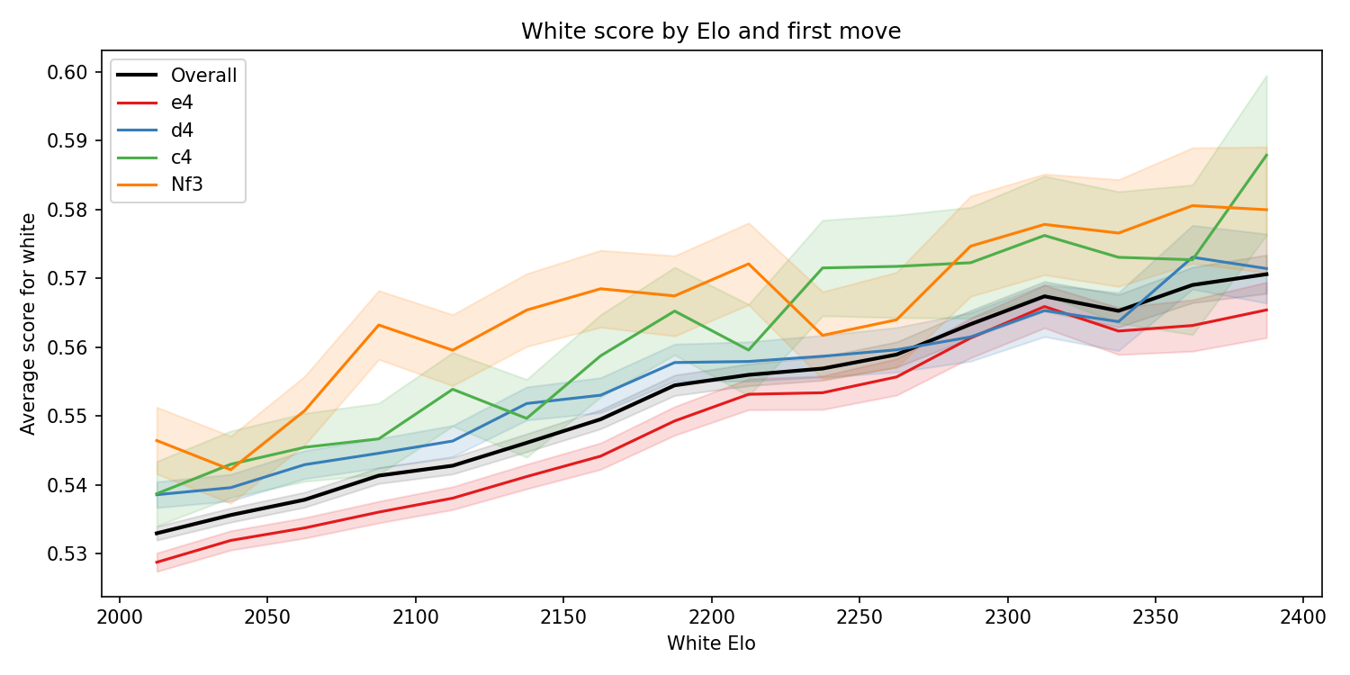
The commenter’s mistake was to not consider the effect sizes.
In particular, matchmaking means that higher rated players play against higher rated opponents, which means that the slope of correlation between Elo and average score on Lichess is small. Look how gentle the upward trend on the graph above is: a 2300 scores just 2.3% points per game more than a 2100.
Additionally, I had already filtered out all games below 2000 Elo, precisely to avoid aggregating over subpopulations that differed too much.
This means that, although the correlations that can cause the Simpson’s paradox are there, they are too weak to explain the data. The Nf3 vs e4 effect is real.
A Second Confounder?
Another commenter hypothesised people choose Nf3 more often against weak opponents:
…maybe people tend [to] use it [Nf3] against lower rated players, so the stats reflect that Black is lower rated, not that White’s position is good?
Much like the previous comment, this also suggests that the players’ ratings are correlating with white’s first move, and therefore the first move is not causal for the better winrate.
Unlike the Simpson’s effect, it hadn’t occurred to me there might be any systematic bias here, so I hadn’t tried to estimate its size.
There’s always more to discover by peeling another layer of the onion, so I investigated. I set out to exactly measure the effect sizes for both these possible confounders.
Separating the Factors
My plan was as follows: Take all white games played by 2000+ players in January 2026, look at how the distribution of white Elo, black Elo, and results differs between e4 and Nf3.
We are going to measure the contributions to the winrate gap from three factors:
White player strength: Nf3 is more popular among stronger players, who win more regardless of opening.
Opponent-based selection: whether the ratio of Nf3 and e4 games changes depending on the opponent Elo.
Move quality: the part that’s left — the genuine advantage from the move.
To measure the size of each effect, we ask counterfactual questions. For example, to isolate the white player strength effect, we ask: “What if Nf3 were played at the same proportions across rating levels as e4, but everything else stayed the same? How much would the winrate gap change?”
Concretely, we divide games into bins by white’s Elo and by the Elo gap between the players. With narrow enough bins, the remaining winrate difference between the openings in each bin can’t be due to correlations with player ratings — it must be the opening itself.
We then use the bins to re-weight: we can take Nf3’s winrate in each bin but pretend the games were distributed across bins the way e4’s games are. This gives us Nf3’s winrate as if it were played by the same relative player strengths as in the e4 games. In other words, we have controlled for player Elos, and the difference is the move quality effect.2
But before I did that, I found a different, more important bias in the data Lichess opening explorer provides, that everyone - including me - had missed. I’ve never seen it discussed.
The Bias We All Missed
Lichess divides the opening database up into rating buckets. The buckets go every 200 Elo, e.g. 2000-2200, 2200-2400 etc. They simply take the average Elo for the game, and put the game in the appropriate bucket. This ensures every game lands neatly into exactly one bucket.
There’s one thing a bit weird about this. If a player is near a boundary, say around 2000 Elo, their games where they played up rating are in one bucket, and their games where they played down rating are in another bucket.
It’s natural to just take this for granted (I and my readers all did), but it introduces a strange filter on whether a particular game by a player makes it in. In our data, when white is around 2000, Lichess is including a lot more games played up-rating than played down-rating.
Which means we are filtering based on something correlated with the outcome we are measuring. That’s a big problem.
When doing my own filtering, I just looked at games played by a white player rated 2000+. This dataset will accurately reflect the average scores of players in that rating range with the white pieces. This is more appropriate, because we want to try to figure out, when a player chooses different first moves, what the effect on all of their results is.
But compared to the Lichess database, we’ve removed some games with 1900s players playing up-rating with white, and added a bunch with 2000s rated players playing down-rating.
This will lift the average scores for all white moves. But it has a bigger effect on e4, because a greater proportion of the games with e4 are played by players near the boundary. Unlike the confounders we are investigating, this isn’t a correlation in the data distribution, but a selection bias on the results we see in the Lichess database.3
This makes a noticeable difference. The average score for 1.e4 is now up to 54.1%, and the average score for 1.Nf3 is 56.2%.4
So with correct filtering the gap between the two moves is 2.1%.
Results: What Causes the Gap?
Now we’ve corrected our data, we can perform our analysis. Here’s what we find:
Move quality is the biggest factor, responsible for a winrate difference of 1.5%.
The factor of white’s rating - i.e. the Simpson’s effect - is 5 times smaller than move quality. It’s responsible for 0.3% of the difference.5
Finally opponent selection is responsible for almost as much: 0.29%. This is still relatively small, but definitely more than I had expected to see.
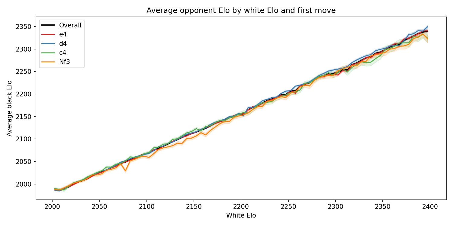
We can actually see the tendency to play Nf3 against weaker opponents if we graph black Elo against white Elo for each first move. The effect seems to be most noticeable around the ~2050-2200 Elo range:
Robustness
The headline result of a 1.5% move quality bonus is robust to experiment design choices. I tested the effect of: how many bins are used; whether to use even width bins or adaptively change them to ensure higher sample counts per bin in the tails; and whether to remove games with Elo differences above some threshold. Nothing I tested changed the move quality estimate by more than 0.05%.
One thing the robustness analysis did show is that the opponent selection effect is almost entirely driven by games played with quite extreme Elo gaps. If we exclude the games with a rating difference over 300, then the opponent selection effect’s size is reduced to just 0.08%.
Conclusion
After controlling for confounders, and more importantly correcting the bias from our filtering, we have a revised effect size of 1.5%. Using the methods from last time, that means we estimate Nf3 to give a boost of about 22 Elo in white games, and a rating increase of 11 Elo overall.
I don’t think this changes my takeaways from the study much. It’s still a small change, but also not negligible. As such, I think database winrates are worth considering in opening choices, but shouldn’t be the driving factor.
The big takeaway from this post is the large effect of the Lichess filters. We should be wary of comparing our results to the statistics from the Lichess opening explorer.
For example, as a 2100, if you are scoring 53% with white, you might think you are doing better than a typical player at your rating, because the Lichess database says white scores 52.5% on average. But with the correct filtering, you can see that 2100s actually score 54.2% with white.
And regarding Nf3 vs e4, we know that there’s something going on that is not explained by how strong the players are, and we know how big it is. But the key question that remains is, what about Nf3 makes it score better?
I have some ideas, but for now I am satisfied to have shown that the effect is real.
I had already thought about this effect, and by a back-of-the-envelope calculation concluded it wasn’t much. The calculation was as follows:
First I looked up a few players rated about 2200, and a few players rated about 2000. The 2200 rated players I checked were winning about 54% of their games on average because they play slightly down-rating. The 2000 rated players were winning 50%.
When you aggregate the 2000 and 2200 buckets, about 1 in 4 e4 games come from the 2200 bucket, but a higher proportion - 1 in 3 - come from Nf3.
Using these proportions for weighted averages of the winrates for players at different Elos means we’d expect 51% winrate for e4, and 51.33% for Nf3.
So the effect in Simpson’s paradox should be accounting for about a 0.33% difference in results.
Because the effects aren’t fully independent, to give a fair attribution we average over the different orders of applying them (i.e. use Shapley Values).
To be clear, I’m not saying the Lichess binning method is wrong, so much as not suitable for our purposes. They have requirements around user experience to factor into their design.
d4 is at 55.0% and c4 at 55.5%; the rank ordering has not changed.
Pleasingly, very close to what my back of the envelope calculation had estimated.